模型训练中防止过拟合的十大实用方案

贺公子之数据科学与艺术

发布于 2026-06-18 11:00:57

1030

1. 什么是过拟合？

过拟合（Overfitting）是机器学习模型训练过程中常见的问题，指模型在训练数据上表现优异，但在未见过的测试数据上表现不佳的现象。简单来说，模型“记住了”训练数据的细节和噪声，而不是学习到数据背后的通用规律。

过拟合的典型表现：

训练集准确率很高（接近100%）
验证集/测试集准确率明显下降
模型对训练数据中的噪声过度敏感
模型复杂度远高于问题本身所需

2. 数据层面的解决方案

2.1 增加训练数据量

数据是机器学习的基础，更多的数据意味着模型能学习到更全面的模式。

实践建议：

收集更多真实数据
使用数据增强技术（特别是计算机视觉任务）
考虑迁移学习，利用预训练模型

2.2 数据增强（Data Augmentation）

通过对现有数据进行变换，生成新的训练样本。

常见的数据增强方法：

图像数据：旋转、翻转、缩放、裁剪、颜色变换
文本数据：同义词替换、随机删除、回译
音频数据：添加噪声、变速、变调

# 图像数据增强示例（使用albumentations库）
import albumentations as A

transform = A.Compose([
    A.RandomRotate90(),
    A.Flip(),
    A.Transpose(),
    A.RandomBrightnessContrast(p=0.5),
    A.RandomGamma(p=0.5),
])

2.3 特征选择与降维

移除冗余或不相关的特征，降低模型复杂度。

常用方法：

主成分分析（PCA）
线性判别分析（LDA）
基于树模型的特征重要性评估
递归特征消除（RFE）

3. 模型层面的解决方案

3.1 正则化技术

正则化通过在损失函数中添加惩罚项，限制模型参数的大小。

L1正则化（Lasso）

惩罚项：λ∑|w|
特点：会产生稀疏解，可用于特征选择

L2正则化（Ridge）

惩罚项：λ∑w²
特点：使权重趋于较小值，但不为零

Elastic Net

结合L1和L2正则化
公式：λ₁∑|w| + λ₂∑w²

# TensorFlow/Keras中的正则化示例
from tensorflow.keras import regularizers

model = tf.keras.Sequential([
    tf.keras.layers.Dense(64, 
                         kernel_regularizer=regularizers.l2(0.01),
                         activity_regularizer=regularizers.l1(0.01)),
    tf.keras.layers.Dense(10)
])

3.2 Dropout

在训练过程中随机“丢弃”一部分神经元，防止神经元之间过度依赖。

Dropout的优势：

相当于训练多个不同的子网络
提高模型的泛化能力
实现简单，效果显著

# Dropout层使用示例
model = tf.keras.Sequential([
    tf.keras.layers.Dense(128, activation='relu'),
    tf.keras.layers.Dropout(0.5),  # 丢弃50%的神经元
    tf.keras.layers.Dense(64, activation='relu'),
    tf.keras.layers.Dropout(0.3),  # 丢弃30%的神经元
    tf.keras.layers.Dense(10, activation='softmax')
])

3.3 早停法（Early Stopping）

监控验证集性能，当性能不再提升时停止训练。

实现要点：

设置合理的耐心值（patience）
保存最佳模型权重
结合学习率调度使用效果更佳

# Early Stopping回调示例
from tensorflow.keras.callbacks import EarlyStopping

early_stopping = EarlyStopping(
    monitor='val_loss',
    patience=10,          # 连续10个epoch验证损失不改善则停止
    restore_best_weights=True,  # 恢复最佳权重
    verbose=1
)

model.fit(X_train, y_train,
          validation_data=(X_val, y_val),
          epochs=100,
          callbacks=[early_stopping])

3.4 批量归一化（Batch Normalization）

对每一层的输入进行归一化处理，加速训练并提高泛化能力。

BN层的作用：

减少内部协变量偏移
允许使用更高的学习率
有一定的正则化效果

4. 训练策略层面的解决方案

4.1 交叉验证（Cross-Validation）

将数据集分成多个子集，轮流作为验证集。

常用方法：

K折交叉验证（K-Fold CV）
留一法交叉验证（Leave-One-Out）
分层K折交叉验证（Stratified K-Fold）

# 5折交叉验证示例
from sklearn.model_selection import cross_val_score
from sklearn.ensemble import RandomForestClassifier

model = RandomForestClassifier(n_estimators=100)
scores = cross_val_score(model, X, y, cv=5, scoring='accuracy')
print(f"交叉验证准确率: {scores.mean():.3f} (±{scores.std():.3f})")

4.2 集成学习（Ensemble Learning）

结合多个模型的预测结果，降低过拟合风险。

常用集成方法：

Bagging：并行训练多个模型，投票或平均
Boosting：顺序训练，关注前序模型的错误
Stacking：用元模型组合多个基模型的预测

4.3 学习率调度

动态调整学习率，帮助模型跳出局部最优。

常用调度策略：

指数衰减
余弦退火
ReduceLROnPlateau（在平台期降低学习率）

5. 模型架构层面的解决方案

5.1 简化模型复杂度

减少网络层数
减少每层的神经元数量
使用更简单的模型架构

5.2 权重约束

限制权重的最大值，防止权重过大。

# 权重约束示例
from tensorflow.keras.constraints import max_norm

model.add(Dense(64, 
                kernel_constraint=max_norm(3.0),  # 限制权重最大范数为3
                activation='relu'))

6. 评估与监控

6.1 学习曲线分析

通过绘制训练和验证损失曲线，直观判断过拟合。

过拟合的典型学习曲线：

训练损失持续下降
验证损失先降后升（出现"U"形）
训练和验证损失差距逐渐增大

6.2 混淆矩阵与分类报告

深入分析模型在各类别上的表现。

6.3 特征重要性分析

理解模型依赖哪些特征做决策。

7. 实践建议与组合策略

7.1 针对不同场景的推荐方案

以下是过拟合解决方案的选择流程图，描述了从数据检查、模型选择到策略组合的完整决策路径：

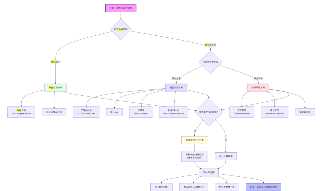
场景类型	推荐方案	理由
小样本数据	数据增强 + Dropout + 早停法	弥补数据不足，防止过拟合
高维特征	L1正则化 + 特征选择	减少特征维度，提高泛化
深度神经网络	Dropout + BN层 + 权重衰减	综合应对深度网络过拟合
传统机器学习	交叉验证 + 集成学习	稳定评估，提高泛化

7.2 组合使用多个方案

在实际项目中，通常需要组合使用多种技术：

# 综合防过拟合策略示例
def create_robust_model(input_shape, num_classes):
    model = tf.keras.Sequential([
        # 输入层
        tf.keras.layers.Input(shape=input_shape),
        
        # 第一层：Dense + BN + Dropout
        tf.keras.layers.Dense(256, 
                             kernel_regularizer=tf.keras.regularizers.l2(0.01)),
        tf.keras.layers.BatchNormalization(),
        tf.keras.layers.Activation('relu'),
        tf.keras.layers.Dropout(0.3),
        
        # 第二层
        tf.keras.layers.Dense(128,
                             kernel_regularizer=tf.keras.regularizers.l2(0.01)),
        tf.keras.layers.BatchNormalization(),
        tf.keras.layers.Activation('relu'),
        tf.keras.layers.Dropout(0.3),
        
        # 输出层
        tf.keras.layers.Dense(num_classes, activation='softmax')
    ])
    
    return model

# 训练配置
callbacks = [
    tf.keras.callbacks.EarlyStopping(patience=10, restore_best_weights=True),
    tf.keras.callbacks.ReduceLROnPlateau(factor=0.5, patience=5)
]

下面是一个完整的端到端实战示例，包含数据生成、模型构建、训练、评估和过拟合对比：

import numpy as np
import matplotlib.pyplot as plt
import tensorflow as tf
from sklearn.datasets import make_classification
from sklearn.model_selection import train_test_split
from sklearn.preprocessing import StandardScaler

# 1. 数据加载与预处理
print("1. 生成模拟数据...")
X, y = make_classification(
    n_samples=5000,          # 总样本数
    n_features=20,           # 特征数
    n_informative=15,        # 有效特征数
    n_redundant=5,           # 冗余特征数
    n_classes=3,             # 类别数
    n_clusters_per_class=2,  # 每类簇数
    random_state=42
)

# 划分训练集、验证集、测试集
X_train, X_temp, y_train, y_temp = train_test_split(X, y, test_size=0.3, random_state=42)
X_val, X_test, y_val, y_test = train_test_split(X_temp, y_temp, test_size=0.5, random_state=42)

# 标准化
scaler = StandardScaler()
X_train = scaler.fit_transform(X_train)
X_val = scaler.transform(X_val)
X_test = scaler.transform(X_test)

print(f"训练集: {X_train.shape}, 验证集: {X_val.shape}, 测试集: {X_test.shape}")

# 2. 模型构建函数（复用前面的 create_robust_model）
def create_robust_model(input_shape, num_classes):
    model = tf.keras.Sequential([
        tf.keras.layers.Input(shape=input_shape),
        
        # 第一层：Dense + L2正则化 + BN + Dropout
        tf.keras.layers.Dense(256, 
                             kernel_regularizer=tf.keras.regularizers.l2(0.01)),
        tf.keras.layers.BatchNormalization(),
        tf.keras.layers.Activation('relu'),
        tf.keras.layers.Dropout(0.3),
        
        # 第二层
        tf.keras.layers.Dense(128,
                             kernel_regularizer=tf.keras.regularizers.l2(0.01)),
        tf.keras.layers.BatchNormalization(),
        tf.keras.layers.Activation('relu'),
        tf.keras.layers.Dropout(0.3),
        
        # 输出层
        tf.keras.layers.Dense(num_classes, activation='softmax')
    ])
    return model

# 3. 创建并编译稳健模型
print("\n2. 构建稳健模型...")
robust_model = create_robust_model(input_shape=(20,), num_classes=3)
robust_model.compile(
    optimizer=tf.keras.optimizers.Adam(learning_rate=0.001),
    loss='sparse_categorical_crossentropy',
    metrics=['accuracy']
)
robust_model.summary()

# 4. 训练配置（早停 + 学习率调度）
callbacks = [
    tf.keras.callbacks.EarlyStopping(
        monitor='val_loss',
        patience=10,
        restore_best_weights=True,
        verbose=1
    ),
    tf.keras.callbacks.ReduceLROnPlateau(
        monitor='val_loss',
        factor=0.5,
        patience=5,
        min_lr=1e-6,
        verbose=1
    ),
    tf.keras.callbacks.ModelCheckpoint(
        'best_robust_model.h5',
        monitor='val_accuracy',
        save_best_only=True,
        verbose=1
    )
]

# 5. 训练稳健模型
print("\n3. 训练稳健模型...")
history_robust = robust_model.fit(
    X_train, y_train,
    validation_data=(X_val, y_val),
    epochs=100,
    batch_size=32,
    callbacks=callbacks,
    verbose=1
)

# 6. 创建过拟合对比模型（无正则化、无Dropout、复杂结构）
print("\n4. 构建过拟合对比模型...")
overfit_model = tf.keras.Sequential([
    tf.keras.layers.Input(shape=(20,)),
    tf.keras.layers.Dense(512, activation='relu'),
    tf.keras.layers.Dense(512, activation='relu'),
    tf.keras.layers.Dense(256, activation='relu'),
    tf.keras.layers.Dense(128, activation='relu'),
    tf.keras.layers.Dense(64, activation='relu'),
    tf.keras.layers.Dense(3, activation='softmax')
])

overfit_model.compile(
    optimizer=tf.keras.optimizers.Adam(learning_rate=0.01),  # 高学习率
    loss='sparse_categorical_crossentropy',
    metrics=['accuracy']
)

# 7. 训练过拟合模型（无早停，小批量）
print("\n5. 训练过拟合模型...")
history_overfit = overfit_model.fit(
    X_train, y_train,
    validation_data=(X_val, y_val),
    epochs=150,  # 更多轮次
    batch_size=8,  # 更小批量，更容易过拟合
    verbose=1
)

# 8. 评估两个模型
print("\n6. 模型评估...")

# 稳健模型评估
robust_train_loss, robust_train_acc = robust_model.evaluate(X_train, y_train, verbose=0)
robust_val_loss, robust_val_acc = robust_model.evaluate(X_val, y_val, verbose=0)
robust_test_loss, robust_test_acc = robust_model.evaluate(X_test, y_test, verbose=0)

print(f"\n稳健模型结果:")
print(f"训练集 - 损失: {robust_train_loss:.4f}, 准确率: {robust_train_acc:.4f}")
print(f"验证集 - 损失: {robust_val_loss:.4f}, 准确率: {robust_val_acc:.4f}")
print(f"测试集 - 损失: {robust_test_loss:.4f}, 准确率: {robust_test_acc:.4f}")

# 过拟合模型评估
overfit_train_loss, overfit_train_acc = overfit_model.evaluate(X_train, y_train, verbose=0)
overfit_val_loss, overfit_val_acc = overfit_model.evaluate(X_val, y_val, verbose=0)
overfit_test_loss, overfit_test_acc = overfit_model.evaluate(X_test, y_test, verbose=0)

print(f"\n过拟合模型结果:")
print(f"训练集 - 损失: {overfit_train_loss:.4f}, 准确率: {overfit_train_acc:.4f}")
print(f"验证集 - 损失: {overfit_val_loss:.4f}, 准确率: {overfit_val_acc:.4f}")
print(f"测试集 - 损失: {overfit_test_loss:.4f}, 准确率: {overfit_test_acc:.4f}")

# 9. 可视化对比
fig, axes = plt.subplots(2, 2, figsize=(14, 10))

# 训练/验证准确率对比
axes[0, 0].plot(history_robust.history['accuracy'], label='稳健模型-训练', color='blue', linestyle='-')
axes[0, 0].plot(history_robust.history['val_accuracy'], label='稳健模型-验证', color='blue', linestyle='--')
axes[0, 0].plot(history_overfit.history['accuracy'], label='过拟合模型-训练', color='red', linestyle='-')
axes[0, 0].plot(history_overfit.history['val_accuracy'], label='过拟合模型-验证', color='red', linestyle='--')
axes[0, 0].set_xlabel('Epoch')
axes[0, 0].set_ylabel('Accuracy')
axes[0, 0].set_title('训练集 vs 验证集准确率对比')
axes[0, 0].legend()
axes[0, 0].grid(True, alpha=0.3)

# 训练/验证损失对比
axes[0, 1].plot(history_robust.history['loss'], label='稳健模型-训练', color='blue', linestyle='-')
axes[0, 1].plot(history_robust.history['val_loss'], label='稳健模型-验证', color='blue', linestyle='--')
axes[0, 1].plot(history_overfit.history['loss'], label='过拟合模型-训练', color='red', linestyle='-')
axes[0, 1].plot(history_overfit.history['val_loss'], label='过拟合模型-验证', color='red', linestyle='--')
axes[0, 1].set_xlabel('Epoch')
axes[0, 1].set_ylabel('Loss')
axes[0, 1].set_title('训练集 vs 验证集损失对比')
axes[0, 1].legend()
axes[0, 1].grid(True, alpha=0.3)

# 泛化差距可视化
epochs_robust = len(history_robust.history['accuracy'])
epochs_overfit = len(history_overfit.history['accuracy'])

robust_gap = np.array(history_robust.history['accuracy']) - np.array(history_robust.history['val_accuracy'])
overfit_gap = np.array(history_overfit.history['accuracy']) - np.array(history_overfit.history['val_accuracy'])

axes[1, 0].plot(range(epochs_robust), robust_gap, label='稳健模型', color='blue', linewidth=2)
axes[1, 0].plot(range(epochs_overfit), overfit_gap, label='过拟合模型', color='red', linewidth=2)
axes[1, 0].axhline(y=0, color='gray', linestyle='--', alpha=0.5)
axes[1, 0].set_xlabel('Epoch')
axes[1, 0].set_ylabel('训练-验证准确率差距')
axes[1, 0].set_title('泛化差距对比（越小越好）')
axes[1, 0].legend()
axes[1, 0].grid(True, alpha=0.3)

# 最终性能对比
models = ['稳健模型', '过拟合模型']
train_accs = [robust_train_acc, overfit_train_acc]
val_accs = [robust_val_acc, overfit_val_acc]
test_accs = [robust_test_acc, overfit_test_acc]

x = np.arange(len(models))
width = 0.25

axes[1, 1].bar(x - width, train_accs, width, label='训练集', color='lightblue', edgecolor='black')
axes[1, 1].bar(x, val_accs, width, label='验证集', color='lightgreen', edgecolor='black')
axes[1, 1].bar(x + width, test_accs, width, label='测试集', color='lightcoral', edgecolor='black')

axes[1, 1].set_xlabel('模型')
axes[1, 1].set_ylabel('准确率')
axes[1, 1].set_title('最终性能对比')
axes[1, 1].set_xticks(x)
axes[1, 1].set_xticklabels(models)
axes[1, 1].legend()
axes[1, 1].grid(True, alpha=0.3, axis='y')

plt.tight_layout()
plt.savefig('overfitting_comparison.png', dpi=300, bbox_inches='tight')
plt.show()

print("\n7. 分析总结:")
print("-" * 50)
print("稳健模型特点:")
print("1. 使用L2正则化、Dropout、BatchNorm等防过拟合技术")
print("2. 配合早停法和学习率调度")
print("3. 训练集和验证集性能接近，泛化差距小")
print("4. 在测试集上表现稳定")

print("\n过拟合模型特点:")
print("1. 网络层数多、神经元多，无正则化")
print("2. 使用高学习率、小批量")
print("3. 训练集准确率高但验证集/测试集差")
print("4. 明显的训练-验证性能差距")

print("\n关键观察:")
print(f"• 稳健模型泛化差距: {robust_gap[-1]:.4f}")
print(f"• 过拟合模型泛化差距: {overfit_gap[-1]:.4f}")
print(f"• 稳健模型在测试集上比过拟合模型高 {100*(robust_test_acc - overfit_test_acc):.2f}%")

运行说明：