Cellchat版本升级?V3空转细胞通讯分析解读

Cellchat版本升级?V3空转细胞通讯分析解读

KS科研分享与服务-TS的美梦
发布于 2026-05-11 15:08:30
发布于 2026-05-11 15:08:30
1、简介并安装包
cellchat更新到V3了?定睛一看,其实不是cellchat版本的更迭,是单独把空转通讯分析单分出来,包的名字是SpatialCellChat。整体的分析流程思路与scRNA的cellchat流程类似。官网提供了详细的流程,这里测试一下流程,让分析使用更加清晰。相比于scRNA,SpatialCellChat的输入除了spot x gene表达矩阵之外,还需要空转spot位置信息,通过整合基因表达、空间距离以及信号配体、受体及其辅助因子之间相互作用的先验知识,来模拟细胞间通讯的概率。在推断出细胞间通讯网络后,SpatialCellChat的各种功能可用于进一步的数据探索、分析和可视化。
Github:https://github.com/jinworks/CellChat
安装SpatialCellChat的时候可以先运行安装,缺少哪些依赖会报错提示,安装好依赖包之后安装SpatialCellChat就没有问题了。
#devtools::install_github("JEFworks-Lab/MERINGUE")
#devtools::install_github("KlugerLab/ALRA")
#BiocManager::install("BiocNeighbors")
#devtools::install_github("zdebruine/RcppML")
#devtools::install_github("jinworks/SpatialCellChat")library(SpatialCellChat)
library(CellChat)
library(Seurat)
library(Matrix)
library(patchwork)
library(ggplot2)
library(dplyr)2、关于输入数据的问题
输入数据要求:从空间转录组数据推断空间分辨的细胞间通讯时,需要提供spot/cell质心的空间坐标/位置。此外,为了过滤掉超出分子最大扩散范围(例如约 250 微米)的细胞间通讯,SpatialCellChat 需要以微米为单位计算细胞质心到质心的距离。因此,对于仅提供像素空间坐标的空转技术,CellChat 通过输入转换因子将空间坐标从像素转换为微米。
data.input (Gene expression data of spots/cells): 表达矩阵,行是基因,列是cell/spots id。矩阵数据要求是Normalized data,如果你提供的是原始矩阵,可以使用CellChat::normalizeData函数进行归一化以及log转化。
meta (User assigned cell labels and samples labels):数据框,行是表达矩阵中对应spot/cell id,包含注释信息,例如cell label,分组信息等,也就是seurat中的metadata。如果是多样本数据,需要有一列标注“sample”的列。不同条件的数据,需要分开分别进行分析。
coordinates (Spatial coordinates of spots/cells): 数据框,cell/spot空间坐标。
spatial.factors (Spatial factors of spatial distance): 一个包含两个距离因素 ratio 和 tol 的数据框,这取决于空间转录组学技术(以及特定的数据集)。(i)ratio:将空间坐标从像素或其他单位转换为微米时的转换因子。例如,设置ratio = 0.18表示在坐标中1像素等于 0.18微米。(ii)tol:在将中心到中心的距离与交互范围进行比较时增加稳健性的容差因子。这可以是cell/spot大小的一半值,单位为微米。不同空间转录组学技术数据集的设置不同,参照https://htmlpreview.github.io/?https://github.com/jinworks/CellChat/blob/master/tutorial/FAQ_on_applying_CellChat_to_spatial_transcriptomics_data.html#x-visium.
contact.range:这个参数在以下情况设置,当在computeCommunProb中通过设定contact.dependent = TRUE推断接触依赖或邻接(juxtacrine)信号,并且使用来自CellChatDB𝑖𝑛𝑡𝑒𝑟𝑎𝑐𝑡𝑖𝑜𝑛annotation 中被归类为“Cell-Cell Contact”的配体-受体对时。这个参数用于限制接触依赖信号作用范围的值(单位:µm)。对于单细胞分辨率的空间转录组,contact.range约等于估计的细胞直径(即中心到中心的距离),意味着接触依赖/邻接信号只有在两个细胞接触时才可能发生。通常可取contact.range=10(典型的人类细胞大小)。
3、加载数据构建spataialcellchat object
以下演示为单个空转样本的通讯分析,多个样本需要分别构建,最后进行比较
这里的演示采用官网用的数据,可以从这里下载:https://github.com/jinworks/SpatialCellChat/tree/main/tutorial。数据来源于一篇NC:https://www.nature.com/articles/s41467-023-39020-4#Abs1。数据是已经构建好的seurat object,并对spots完成了cell标注。
load("~/data_analysis/R版decoupleR/spatial_data/visium_human_psoriasis.RData")
SpatialDimPlot(seu, stroke=0.1,pt.size.factor = 3)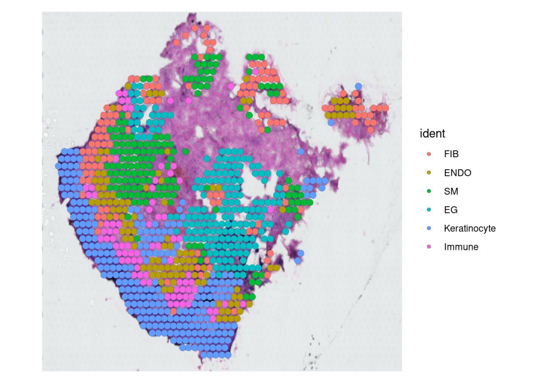
但是这个数据结构有点问题,需要先处理一下,您自己构建好的数据如果已经完成了标准化,没必要进行这些处理。观察seu的结构会发现,它的count layer没有数据,data layer却是count数据,所以需要补一下count并进行标准化处理。
Seurat::DefaultAssay(seu) <- "Spatial" #设置assay
seu@assays$Spatial@counts <- seu@assays$Spatial@data
seu <- Seurat::NormalizeData(seu)
seu## An object of class Seurat
## 33544 features across 905 samples within 2 assays
## Active assay: Spatial (33538 features, 0 variable features)
## 2 layers present: counts, data
## 1 other assay present: predictions
## 2 dimensional reductions calculated: pca, umap
## 1 image present: slice1对于seurat object,只需要准备coordinates和spatial.factors两个参数内容即可,直接可以使用seurat obj构建spatialcellchat object。其他类型的数据需要按照前面所述分别准备matrix表达矩阵,meta等等进行构建。
# prepare spatial transcriptomics information
spatial.locs <- Seurat::GetTissueCoordinates(seu, scale = NULL, cols = c("imagerow", "imagecol"))
# spatial factors of spatial coordinates
scalefactors <- jsonlite::fromJSON(txt = file.path("./spatial_data/scalefactors_json.json"))
spot.size <- 65 # the theoretical spot size (um) in 10X Visium
conversion.factor <- spot.size/scalefactors$spot_diameter_fullres
spatial.factors <- list(ratio = conversion.factor, tol = spot.size/2)chat <- createSpatialCellChat(
object = seu, # Seurat
group.by = "final.clusters",#metadata中cell labels
assay = "Spatial", # normalized
datatype = "spatial",
coordinates = spatial.locs,
spatial.factors = spatial.factors
)4、cellchat分析
解析来的分析步骤与scRNA的cellchat步骤类似。
4.1 设置受配体数据库:
CellChatDB是一个经过人工整理的文献支持的人类和小鼠配体-受体相互作用数据库,CellChatDB v2 包含约3200个经过验证的分子相互作用,CellChatDB将配体-受体对分为不同类别,包括“分泌信号”、“细胞外基质-受体”、“细胞-细胞接触”和“非蛋白信号”。默认情况下,不使用“非蛋白信号”。关于自定义以及数据库更新参考https://mp.weixin.qq.com/s/gH2cwQTDVrAraIiB9i1rwA。
CellChatDB <- CellChatDB.human # use CellChatDB.mouse if running on mouse data
showDatabaseCategory(CellChatDB) #看看数据库组成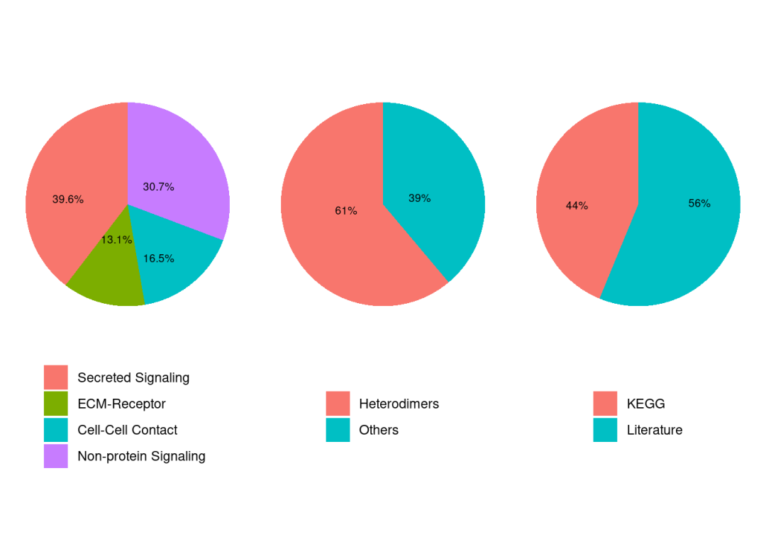
# use a subset of CellChatDB for cell-cell communication analysis
CellChatDB.use <- subsetDB(CellChatDB, search = c("Secreted Signaling", "ECM-Receptor", "Cell-Cell Contact"), non_protein = F)
# CellChatDB.use <- subsetDB(CellChatDB)#使用除non_protein信号的其他信号
#在spataialcellchat object中设置选择的数据库
chat@DB <- CellChatDB.use
4.2 预处理表达数据:
识别空间可变的配体或受体,进而识别空间可变的配体-受体相互作用。
chat <- subsetData(chat) # This step is necessary even if using the whole database
chat <- preProcessing(chat) chat <- SpatialCellChat::identifyOverExpressedGenes(
chat,
selection.method = "meringue"
)chat <- SpatialCellChat::identifyOverExpressedInteractions(
chat,
variable.both = F # only require that either ligand or receptor from one pair is over-expressed
)4.3 推断通讯网络:
SpatialCellChat通过为每个相互作用分配一个概率值并执行置换检验,来推断具有生物学意义的细胞间通讯。SpatialCellChat利用质量作用定律,将基因表达数据与信号配体、受体及其辅助因子之间相互作用的先验知识相结合,同时考虑cell/spots之间的空间距离,从而对细胞间通讯的概率进行建模。
Compute the communication probability and infer cellular communication network at the individual cell level:
chat <- computeCommunProb(
  chat,
  distance.use = TRUE, #是否在计算通信概率时引入距离约束。设为TRUE表示细胞间通信概率与计算得到的空间距离成反比关系。
  scale.distance = 0.2,#参数distance.use设为TRUE时,需要设置scale.distance对空间距离进行缩放或归一化,这个参数不同的数据需要按照实际情况自行设置,可以取值1、0.1、0.01、0.001、0.11等,保证缩放后的最小距离落在[1,2]区间内。
  contact.dependent = TRUE,#是否基于contact.range确定空间上邻近的细胞群,默认True,如果只关注“分泌型信号”,则将自动设置为FALSE。
  interaction.range = 250, #配体的最大作用/扩散距离(单位:微米),该硬性阈值用于过滤掉空间上相距较远的单个细胞之间的连接。
  contact.range = 10#用于限制接触依赖性信号的相互作用范围,通常contact.range = 10,这是典型的人类细胞大小。然而,对于低分辨率的空间数据(如10X Visium),该参数应设置为细胞中心到细胞中心的距离(例如,对于 Visium 数据,contact.range = 100)。computeCellDistance 函数可用于计算细胞中心到中心的距离。
)chat <- filterProbability(chat)
chat <- filterCommunication(
chat,
min.cells = NULL,
min.links = 10,
min.cells.sr = 10
)Infer the communication network at the cell group level:对于低分辨率的空间数据,例如10x visium,可使用computeAvgCommunProb_Visium函数计算细胞群水平的细胞间通讯,并通过参数 cell.type.decomposition 传入细胞类型比例(反卷积结果矩阵)。对于高分辨率数据,使用 computeAvgCommunProb函数。
cell.type.decomposition <- t(seu@assays[["predictions"]]@data)
cell.type.decomposition[cell.type.decomposition<0.1] <- 0
head(cell.type.decomposition)## FIB ENDO SM EG Keratinocyte Immune
## AAACCGGGTAGGTACC-1 0.0000000 0.6756632 0.0000000 0 0 0.2598581
## AAACCGTTCGTCCAGG-1 0.0000000 0.0000000 0.0000000 0 0 1.0000000
## AAACCTCATGAAGTTG-1 0.0000000 0.9485086 0.0000000 0 0 0.0000000
## AAACGAGACGGTTGAT-1 0.1810008 0.1871610 0.5893234 0 0 0.0000000
## AAACTTGCAAACGTAT-1 0.0000000 0.0000000 0.0000000 0 1 0.0000000
## AAAGACTGGGCGCTTT-1 0.9935221 0.0000000 0.0000000 0 0 0.0000000chat <- computeAvgCommunProb_Visium(
chat,
cell.type.decomposition = as.matrix(cell.type.decomposition),
avg.type = 'avg',
nboot = 100,
do.permutation = T
)chat <- filterCommunication(chat, min.cells = 10, min.links = NULL, min.cells.sr = NULL)4.4 提取并保存结果:
这里可以将结果提取出来,使用subsetCommunication函数可以设置source、target以及显著性等等。按照需求进行提取。如果不设置参数,则提取所有结果。
df.net <- subsetCommunication(chat)
head(df.net)
4.5 推断信号通路水平的细胞间通讯:
CellChat通过汇总与每条信号通路相关的所有配体-受体相互作用的通讯概率,计算信号通路水平的通讯概率。注意:每个配体-受体对以及每条信号通路的推断细胞间通讯网络分别存储在 net 槽和 netP 槽中。
chat <- computeCommunProbPathway(chat)4.6 计算聚合的细胞间通讯网络:
通过统计link数量或汇总通讯概率来计算聚合的细胞间通讯网络。还可以通过设置sources.use和 targets.use参数,计算特定细胞群子集之间的聚合网络。
chat <- aggregateNet(chat)5、分析可视化
5.1 一般可视化功能:
SpatialCellChat可以直接对反卷机结果可视化;当然需要是cellchat obj。
SpatialCellChat::spatialDimPlot(chat, proportion = cell.type.decomposition, point.size = 1.5)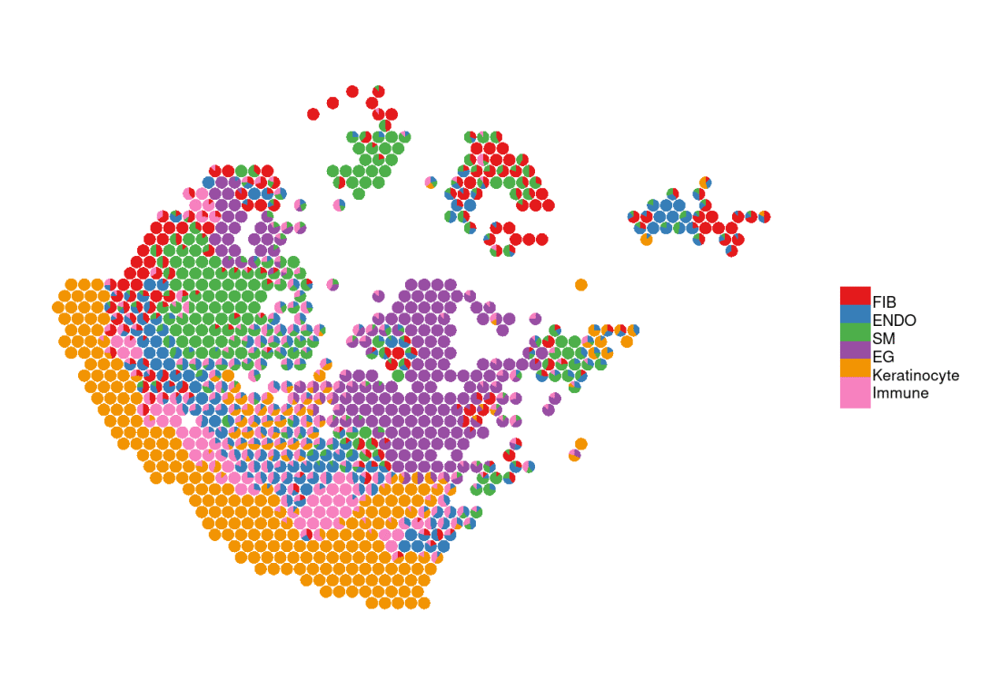
可视化基因表达,提供cellchat通路,可以直接可以画所有通路相关基因的表达:
pathway.show <- "WNT"
# show the expression distributions of genes associated with the specific pathway
spatialFeaturePlot(chat, signaling = pathway.show, do.group = FALSE, do.binary = FALSE, color.heatmap = "Spectral", point.size = 1.3)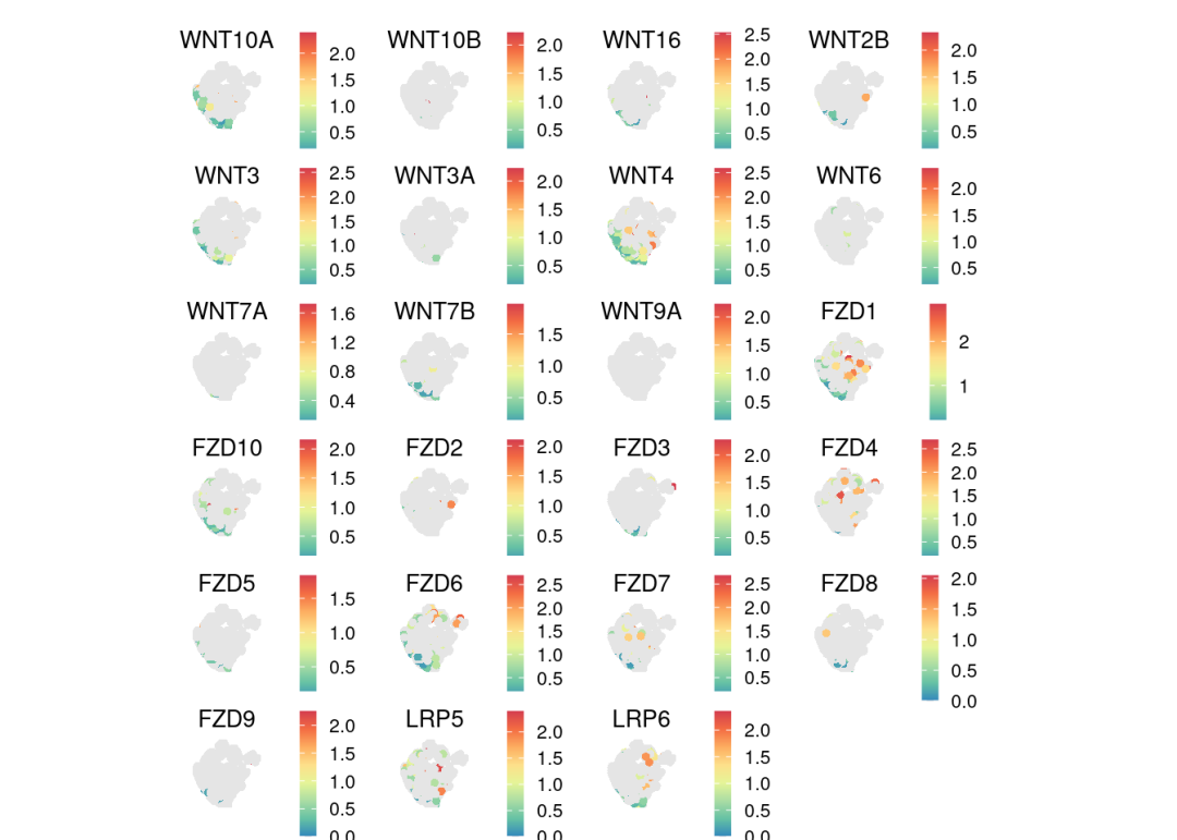
extractEnrichedLR函数用于提取给定信号通路中所有显著的相互作用(配体-受体对)及相关信号传导基因。可以在spatialFeaturePlot中设置do.binary=TRUE,以二值化并可视化特定配体-受体对中配体与受体基因在同一图幅中的表达分布。在这种情况下,必须提供参数 cutoff 作为表达水平的阈值。
# show the expression distributions of genes associated with the specific L-R pair
enrichedLR <- SpatialCellChat::extractEnrichedLR(chat, signaling = 'TNF', do.group = FALSE)
LR.show <- enrichedLR[1,,drop = FALSE] # only show one ligand-receptor pair
SpatialCellChat::spatialFeaturePlot(chat, pairLR.use =  LR.show, do.group = FALSE, do.binary = TRUE, cutoff = 0.05, point.size = 1.5)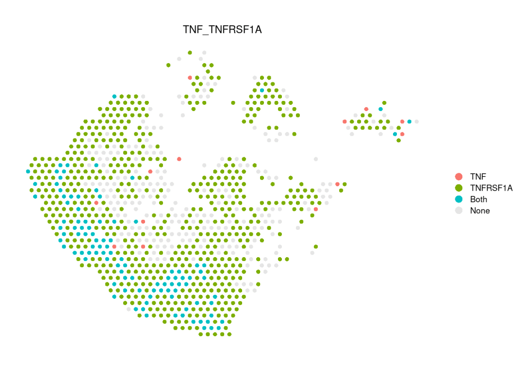
5.2 可视化单个cell/spot水平上推断的细胞间通讯:
计算网络中心性得分:
chat <- netAnalysis_computeCentrality(
  chat,
  slot.name = "net",
  do.group = F,
  degree.only = T
)gg1 <- SpatialCellChat::spatialVisual_scoring(chat, signaling = pathway.show, slot.name = "netP", do.group = FALSE, measure = c("outdeg"), do.binary = FALSE, color.heatmap = "Blues", point.size = 1)
gg2 <- SpatialCellChat::spatialVisual_scoring(chat, signaling = pathway.show, slot.name = "netP", do.group = FALSE, measure = c("indeg"), do.binary = FALSE, color.heatmap = "Reds", point.size = 1)
patchwork::wrap_plots(gg1, gg2, ncol =2)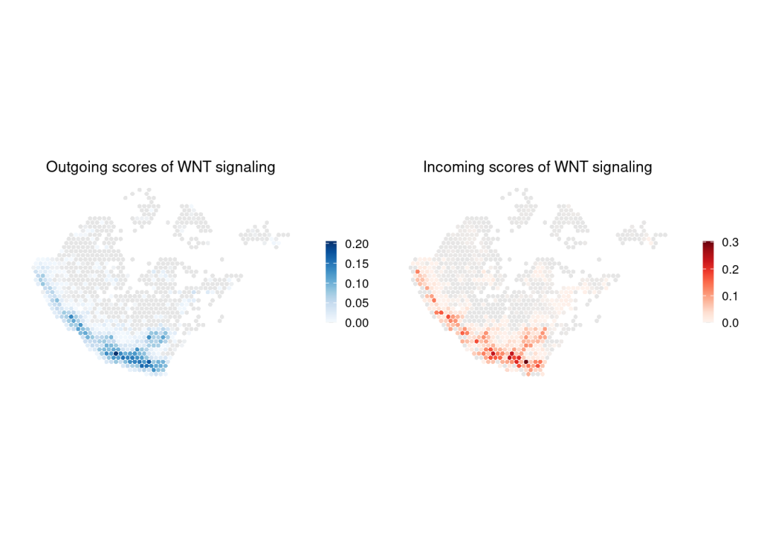
展示配体-受体对的传出与传入评分,
所有显著通讯的配体-受体对均可通过chat@net$LR.sig获取。
LR.show <- chat@net$LR.sig[1]
gg1 <- SpatialCellChat::spatialVisual_scoring(chat, signaling = LR.show, slot.name = "net", do.group = FALSE, measure = c("outdeg"), do.binary = FALSE, color.heatmap = "Blues", point.size = 1)
gg2 <- SpatialCellChat::spatialVisual_scoring(chat, signaling = LR.show, slot.name = "net", do.group = FALSE, measure = c("indeg"), do.binary = FALSE, color.heatmap = "Reds", point.size = 1)
patchwork::wrap_plots(gg1, gg2, ncol =2)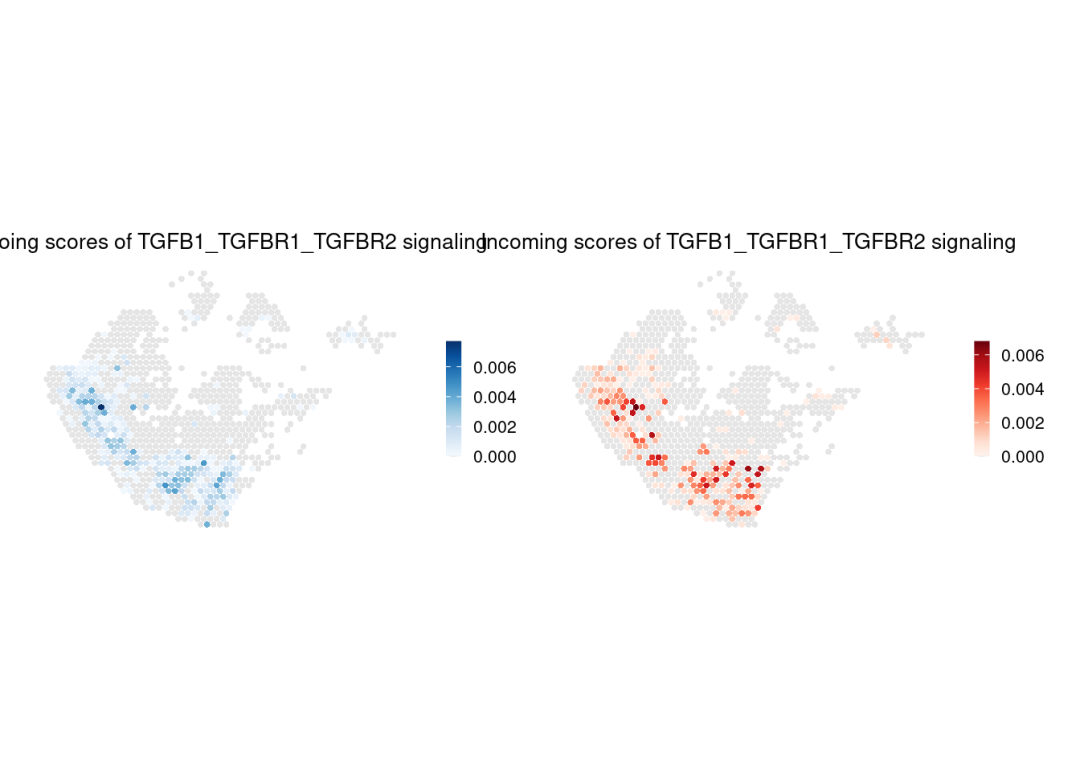
5.3 在cell group水平上可视化推断的细胞间通讯:
类似于scRNA上的可视化,标注出细胞分群,按照细胞群展示通讯网络。
SpatialCellChat::netVisual_aggregate(chat, signaling = pathway.show, layout = "circle")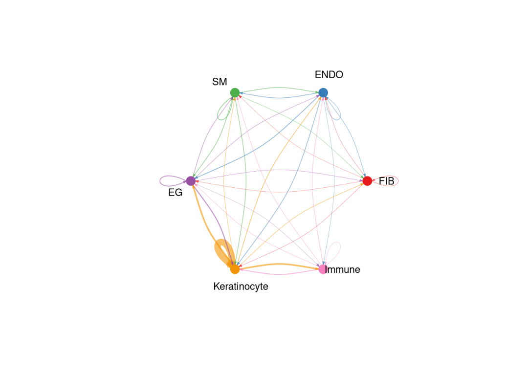
chat <- netAnalysis_computeCentrality(
  chat,
  slot.name = "netP",
  do.group = T,
  degree.only = T
)library(RColorBrewer)
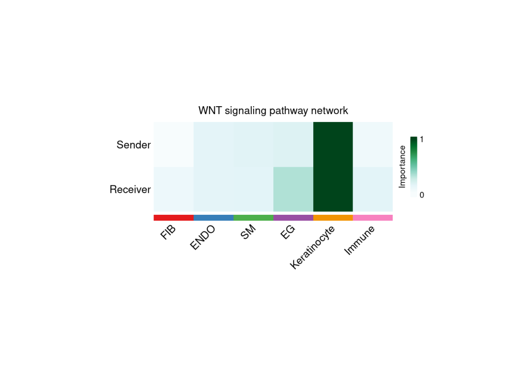
SpatialCellChat::netAnalysis_signalingRole_network(
chat, signaling = pathway.show, slot.name = "netP",
measure = c("outdeg","indeg"), measure.name = c("Sender","Receiver"),
width = 8, height = 3, font.size = 10
)
5.4 识别富集的信号通路:
rankNet函数用于对通讯活跃的信号进行排序。分析信号通路时,设置slot.name=‘netP’;分析配体-受体对时,设置 slot.name = ‘net’。此外,通过 signaling.type 参数指定信号类型,该参数默认为 NULL,表示进行整体排序。同时,可分别使用sources.use和targets.use参数来定义发送细胞群和接收细胞群。
g1 <- SpatialCellChat::rankNet(chat, mode = "single", slot.name = "netP", measure = "weight", signaling.type = "Secreted Signaling",title = "Secreted Signaling")
g2 <- SpatialCellChat::rankNet(chat, mode = "single", slot.name = "netP", measure = "weight", signaling.type = "ECM-Receptor",title = "ECM-Receptor")
g3 <- SpatialCellChat::rankNet(chat, mode = "single", slot.name = "netP", measure = "weight", signaling.type = "Cell-Cell Contact",title = "Cell-Cell Contact")
patchwork::wrap_plots(g1, g2, g3, ncol = 3)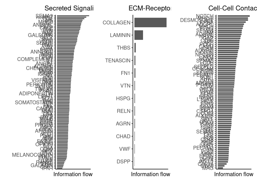
本文参与 腾讯云自媒体同步曝光计划,分享自微信公众号。
原始发表:2026-05-10,如有侵权请联系 cloudcommunity@tencent.com 删除
评论
登录后参与评论
推荐阅读
目录
腾讯云开发者

Copyright © 2013 - 2026 Tencent Cloud. All Rights Reserved. 腾讯云 版权所有
深圳市腾讯计算机系统有限公司 ICP备案/许可证号:粤B2-20090059 ![]() 粤公网安备44030502008569号
粤公网安备44030502008569号
腾讯云计算(北京)有限责任公司 京ICP证150476号 | 京ICP备11018762号