执行计划跑偏,你了解背后的根因吗?

执行计划跑偏,你了解背后的根因吗?

NickYoung
发布于 2026-07-09 16:34:13
发布于 2026-07-09 16:34:13
还在以最终cost来判断计划是否最优?那就大错特错了!!!本篇老杨和大家一起抽丝剥茧,从源码入手分析计划跑偏的原因。
问题现象
一个简单查询运行240s,从执行计划看耗时主要在nestloop join,Outter扫描了2293行,inner loop扫描了2293次,耗时103.1 * 2293 = 236408ms
test=> explain analyze select count(*),zone_id from instance_info where instanceid in (SELECT instanceid
FROM
    instance_info
wherevisible = 1
GROUPBY
    instanceid
HAVING
    COUNT(DISTINCT zone_id) > 1) andvisible = 1groupby zone_id;
                                                                   QUERY PLAN
-------------------------------------------------------------------------------------------------------------------------------------------------
 GroupAggregate  (cost=232.45..232.47 rows=1 width=12) (actual time=244941.317..244942.725 rows=4.00 loops=1)
   Group Key: instance_info.zone_id
   Buffers: shared hit=3
   ->  Sort  (cost=232.45..232.45 rows=1 width=4) (actual time=244940.890..244941.590 rows=4588.00 loops=1)
         Sort Key: instance_info.zone_id
         Sort Method: quicksort  Memory: 193kB
         Buffers: shared hit=3
         ->  Nested Loop  (cost=200.01..232.44 rows=1 width=4) (actual time=124.292..244935.769 rows=4588.00 loops=1)
               Join Filter: ((instance_info.instanceid)::text = (instance_info_1.instanceid)::text)
               Rows Removed by Join Filter: 20185277
               ->  Foreign Scan  (cost=100.01..116.12 rows=1 width=146) (actual time=25.421..137.939 rows=2293.00 loops=1)
                     Relations: Aggregate on (instance_info instance_info_1)
               ->  Foreign Scan on instance_info  (cost=100.00..116.30 rows=2 width=150) (actual time=1.290..103.183 rows=8805.00 loops=2293)
 Planning:
   Buffers: shared hit=173
 Planning Time: 1.516 ms
 Execution Time: 244953.762 ms
(17 rows)

test=>
一般遇到这种情况,肯定是尝试“关闭”nestloop试试看,走了Hashjoin后执行耗时仅287ms,性能提升快1000倍。
test=> set enable_nestloop tooff;
SET
test=> explain analyze select count(*),zone_id from instance_info where instanceid in (SELECT instanceid
FROM
    instance_info
wherevisible = 1
GROUPBY
    instanceid
HAVING
    COUNT(DISTINCT zone_id) > 1) andvisible = 1groupby zone_id;
                                                                  QUERY PLAN
----------------------------------------------------------------------------------------------------------------------------------------------
 GroupAggregate  (cost=232.44..232.46 rows=1 width=12) (actual time=273.475..274.907 rows=4.00 loops=1)
   Group Key: instance_info.zone_id
   Buffers: shared hit=3
   ->  Sort  (cost=232.44..232.45 rows=1 width=4) (actual time=273.006..273.722 rows=4588.00 loops=1)
         Sort Key: instance_info.zone_id
         Sort Method: quicksort  Memory: 193kB
         Buffers: shared hit=3
         ->  Hash Join  (cost=216.13..232.43 rows=1 width=4) (actual time=160.901..271.843 rows=4588.00 loops=1)
               Hash Cond: ((instance_info.instanceid)::text = (instance_info_1.instanceid)::text)
               ->  Foreign Scan on instance_info  (cost=100.00..116.30 rows=2 width=150) (actual time=4.691..109.722 rows=8805.00 loops=1)
               ->  Hash  (cost=116.12..116.12 rows=1 width=146) (actual time=156.185..156.186 rows=2293.00 loops=1)
                     Buckets: 4096 (originally 1024)  Batches: 1 (originally 1)  Memory Usage: 144kB
                     ->  Foreign Scan  (cost=100.01..116.12 rows=1 width=146) (actual time=21.939..155.037 rows=2293.00 loops=1)
                           Relations: Aggregate on (instance_info instance_info_1)
 Planning Time: 0.242 ms
 Execution Time: 287.414 ms
(16 rows)

test=>
为什么优化器走了效率更差的nested loop?
统计信息不准?优化器代价计算偏差?
问题分析
从nestloop和Hashjoin对应path的最终cost来看
GroupAggregate (cost=232.45..232.47)
GroupAggregate (cost=232.44..232.46)
后者对应path最终的startup_cost和total_cost都要小,为什么优化器没有选择Hashjoin这条路径?
所以这里会有一个误区:老杨也曾以为优化器选择最优执行计划,肯定是生成每种路径后,比较最终的cost,最终cost最小的为最优计划。
事实上在add_path生成路径的过程中,每个节点都会进行cost比较,可能采用new_path,或者保留old_path,或者都保留。比如说在生成Joinpath时,可能只保留了一种JoinMethod进入下一计划节点,生成最终执行计划。
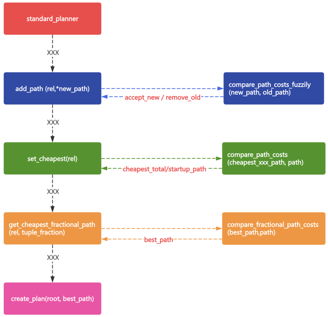
那么这个案例中有没有可能是Hashjoin在Joinpath环节被“淘汰了”?
Nested Loop (cost=200.01..232.44 rows=1 width=4)
Hash Join (cost=216.13..232.43 rows=1 width=4)
从cost来看,两种路径的cost比较接近,由于之前研究过这里,我已经大概猜到问题的原因了。
在add_path生成路径时,首先使用模糊cost比较来决定路径的去留。
cost模糊比较函数为compare_path_costs_fuzzily[1]:
path1即new_path为HashPath,path2 即old_path为NestPath。
- 首先比较两条路径的disabled_nodes。 enable_nestloop和enable_hashjoin均为on,所以disabled_nodes均为0。
- 若未果,再比较total_cost,并通过模糊系数将路径cost提升1%,和另外一条路径比较; 232.43 > 232.44 * 1.01 和 232.44 > 232.43 * 1.01均不成立,total_cost模糊近似。
- 若未果,再比较startup_cost,并通过模糊系数将路径cost提升1%,和另外一条路径比较 216.13 > 200.01 * 1.01所以返回COSTS_BETTER2。
经过比较确定两条路径中更优路径为NestPath。 那么HashPath就被淘汰了,然后进行后续SORT和AGG节点的path生成。
static PathCostComparison
compare_path_costs_fuzzily(Path *path1, Path *path2, double fuzz_factor)
{
#define CONSIDER_PATH_STARTUP_COST(p)  \
 ((p)->param_info == NULL ? (p)->parent->consider_startup : (p)->parent->consider_param_startup)

/* Number of disabled nodes, if different, trumps all else. */
if (unlikely(path1->disabled_nodes != path2->disabled_nodes))
 {
if (path1->disabled_nodes < path2->disabled_nodes)
   return COSTS_BETTER1;
else
   return COSTS_BETTER2;
 }

/*
  * Check total cost first since it's more likely to be different; many
  * paths have zero startup cost.
  */
if (path1->total_cost > path2->total_cost * fuzz_factor)
 {
/* path1 fuzzily worse on total cost */
if (CONSIDER_PATH_STARTUP_COST(path1) &&
   path2->startup_cost > path1->startup_cost * fuzz_factor)
  {
   /* ... but path2 fuzzily worse on startup, so DIFFERENT */
   return COSTS_DIFFERENT;
  }
/* else path2 dominates */
return COSTS_BETTER2;
 }
if (path2->total_cost > path1->total_cost * fuzz_factor)
 {
/* path2 fuzzily worse on total cost */
if (CONSIDER_PATH_STARTUP_COST(path2) &&
   path1->startup_cost > path2->startup_cost * fuzz_factor)
  {
   /* ... but path1 fuzzily worse on startup, so DIFFERENT */
   return COSTS_DIFFERENT;
  }
/* else path1 dominates */
return COSTS_BETTER1;
 }
/* fuzzily the same on total cost ... */
if (path1->startup_cost > path2->startup_cost * fuzz_factor)
 {
/* ... but path1 fuzzily worse on startup, so path2 wins */
return COSTS_BETTER2;
 }
if (path2->startup_cost > path1->startup_cost * fuzz_factor)
 {
/* ... but path2 fuzzily worse on startup, so path1 wins */
return COSTS_BETTER1;
 }
/* fuzzily the same on both costs */
return COSTS_EQUAL;

#undef CONSIDER_PATH_STARTUP_COST
}
debug做下验证:
在生成Joinpath时,依次生成MergePath、NestPath、HashPath并进行cost模糊比较。
这里省去MergePath和NestPath的比较过程,NestPath胜出。
当生成HashPath后,和NestPath比较Total_cost差异并未达到1%。而进一步比较startup_cost,明显差异大于1%所以返回COSTS_BETTER2,即NestPath胜出。
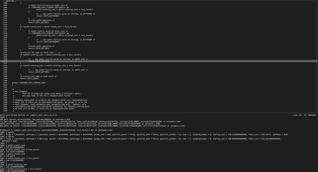
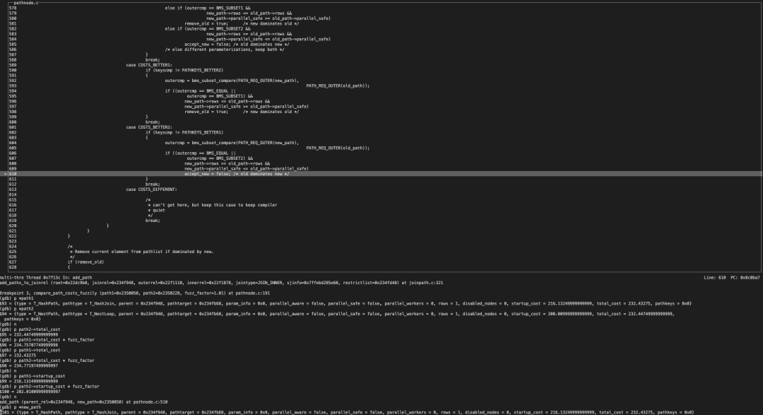
case COSTS_BETTER2:当前满足outercmp == BMS_EQUAL等条件,将accept_new置为false
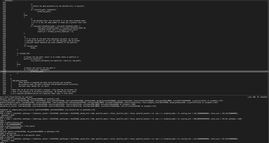
accept_new为false,所以拒绝并且回收了new_path,也就是HashPath被淘汰了。
经过cost精确比较,角逐出cheapest_total_cost和cheapest_startup_cost都为NestPath。
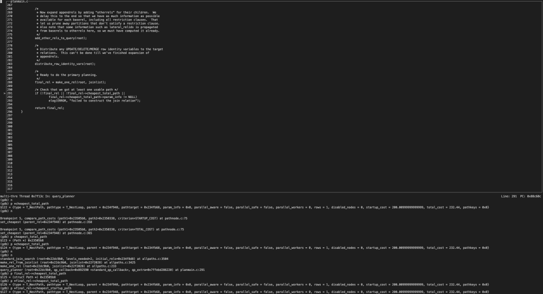
最终,使用best_path去生成执行计划。
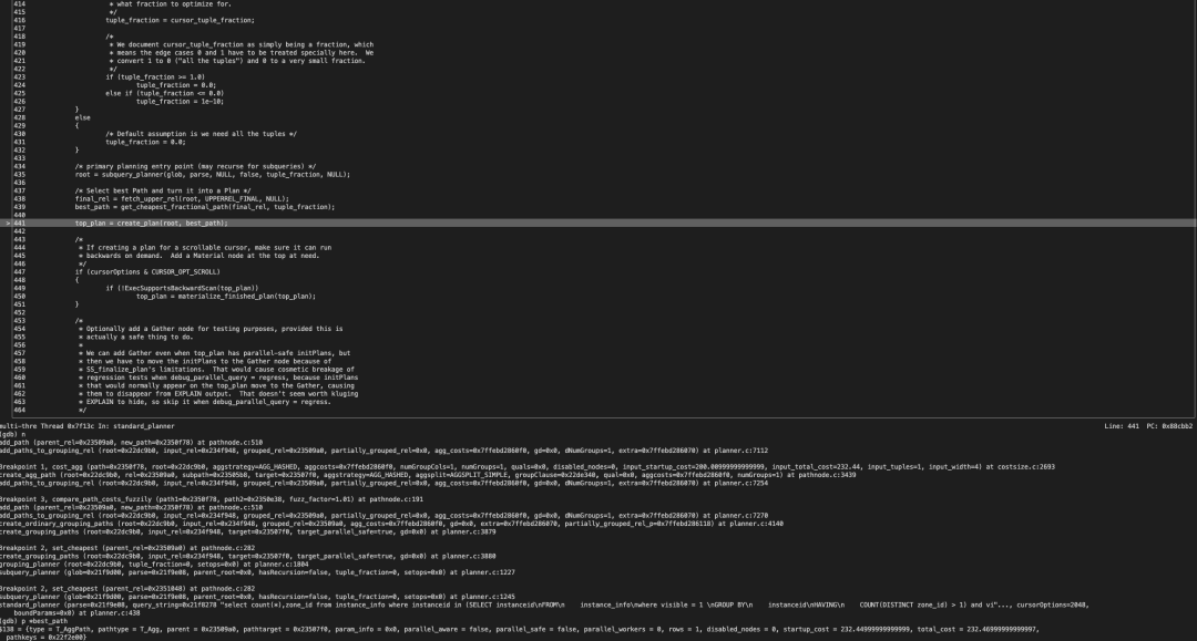
到这里,大家已经感觉到这个cost模糊比较有坑了吧,特别当两条路径的cost差别比较小,total_cost或者startup_cost差别小于1%时,可能会导致选错路径,最终生成了一个次优计划。
STD_FUZZ_FACTOR默认就是1.01,是不是可以把它调整得更小,这样就能更精准?但得慎重,这里也是优化器最核心的部分,弄不好真是牵一发则动全身。我觉得这个模糊比较目前看起来不太优雅,甚至后续版本有可能去除这里的逻辑,当然各位有想法的话可以发到社区和Tom Lane一众大佬solo下。
当然不能指望优化器一直都是最正确的,这是违背现实的,我之前也写了很多篇文章,多次分享相关的内容。
ok,那么为什么这个case走了不优计划,大家应该都清楚了。可能已经有朋友看出来还有点小问题,Foreign table预估扫描1行,实际扫描了2000+行,肯定是统计信息不准啊?
大家思考下Foreign table有统计信息吗?
sure,篇幅问题,我简述下原理:Foreign table只是表映射,没有物理元组,它的统计信息,是通过fdw访问目的端表进行采集的。 但是只能手动挡,因为Foreign table没法进行vacuum/autovacuum,需要手动analyze触发。
示例的表我做了下analyze,更新了下统计信息,各种path的cost差异比较大,默认走了Hashjoin。
因此,一定要定时收集外表统计信息,不然可能会拖垮整个实例。
小结
本篇我们分析了一例执行计划跑偏的根本原因,从中看得到当路径间的cost接近时(1%以下),可能在add_path 时cost模糊比较中会选择次优路径,生成不优计划。
当然遇到这样的场景可以尝试各种hint手段去干预,不过可以考虑利用强化学习来实现自动化的hint干预,让数据库自动管理执行计划。我在之前的文章《AI4DB试玩-Bao/Balsa适配PG18》中研究过类似的模型,并在PCC2025大会中做了分享。
当然专业的事要专业的人来做,我们的好友崔鹏博士已有相关的AI4DB课题研究和落地,将会在HOW2026大会中与大家见面,敬请期待。
Reference
[1]
https://github.com/postgres/postgres/blob/REL_18_0/src/backend/optimizer/util/pathnode.c#L185
本文参与 腾讯云自媒体同步曝光计划,分享自微信公众号。
原始发表:2025-12-25,如有侵权请联系 cloudcommunity@tencent.com 删除
目录
腾讯云开发者

Copyright © 2013 - 2026 Tencent Cloud. All Rights Reserved. 腾讯云 版权所有
深圳市腾讯计算机系统有限公司 ICP备案/许可证号:粤B2-20090059  粤公网安备44030502008569号
腾讯云计算(北京)有限责任公司 京ICP证150476号 | 京ICP备11018762号