COMP7801 Topic 1a Relational Database

Relational Databases

Structure of Relational Databases

Basic structure

• Given sets D1, D2, …, Dn
• A relation r is a subset of D1 x D2 x …, x Dn
• A relation is a set of n-tuples (a1, a2, …, an) where each ai Di

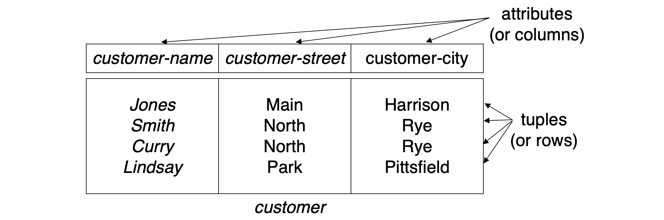
Example

• if
  • customer-name = {Jones, Smith, Curry, Lindsay}
  • customer-street = {Main, North, Park}
  • customer-city = {Harrison, Rye, Pittsfield}
• Then
  • r = {(Jones, Main, Harrison), (Smith, North, Rye), (Curry, North, Rye), (Lindsay, Park, Pittsfield)} is a relation over customer-name x customer-street x customer-city

Attribute Types

• Each attribute of a relation has a name
• The set of allowed values for each attribute is called the domain of the attribute

Relation Schema

• A1, A2, …, An are attributes
• R = (A1, A2, …, An ) is a relation schema
  • E.g. Account-schema = (account-number, branch-name, balance)
• r(R) is a relation on the relation schema R
  • E.g. customer(Customer-schema)

Relation Instance

• The current values (relation instance) of a relation are specified by a table
• An element t of r is a tuple, represented by a row in a table

Database

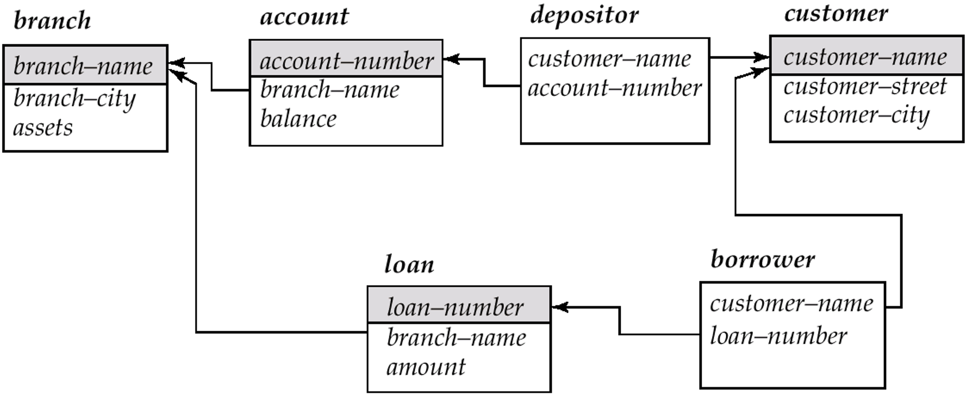
• A database consists of multiple relations which are inter-related
• Information about an enterprise is broken up into parts, with each relation storing one part of the information

Query language

Language in which user requests information from the database

• Categories
  • procedural
  • non-procedural
• Pure languages
  • Relational Algebra
    • The operators take one or more relations as inputs and give a new relation as a result
    • Operations
      • select
      • project
      • union
      • set-Intersection
      • set difference
      • cartesian product
      • rename
      • Natural Join
      • Aggregate Functions
        • avg: average value
        • min: minimum value
        • max: maximum value
        • sum: sum of values
        • count: number of values
  • Relational Calculus

SQL

• SQL is based on set and relational operations with certain modifications and enhancements
• A typical SQL query has the form
  • select A1, A2, ..., Anfrom r1, r2, ..., rm where P
• The result of an SQL query is a multiset of tuples
• Clauses
  • select
    • To force the elimination of duplicates, insert the keyword distinct after select
  • where
    • The where clause specifies conditions that the result must satisfy
      • Comparison results can be combined using the logical connectives and, or, and not
      • Comparisons can be applied to results of arithmetic expressions
  • from
    • The from clause lists the relations involved in the query
• Aggregate Functions
  • Group By
    • Find the number of depositors for each branch
      • select branch-name,count (distinct customer-name)from depositor,account where depositor.account-number = account.account-numbergroup by branch-name
  • Having
    • formation of groups whereas predicates in the where clause are applied before forming groups

Query Evaluation

• Basic operations
  • Selections
  • Joins
  • Other operations (projection, aggregation)
• Transformation of queries into a tree of operations

Query Optimizationh

• Many equivalent expressions to the original query can be derived
• The query optimizer uses statistical data and appropriate algorithms to compute an expression of low evaluation cost

Storage of databases

Physical Storage Media

• Cache
  • fastest and most costly form of storage
  • volatile
  • managed by the computer system hardware
• Main memory
  • fast access
  • generally too small (or too expensive) to store the entire database
  • Volatile
    • contents of main memory are usually lost if a power failure or system crash occurs
• Magnetic-disk
  • Data is stored on spinning disk, and read/written magnetically
  • Primary medium for the long-term storage of data
  • typically stores entire database
  • Data must be moved from disk to main memory for access, and written back for storage
    • Much slower access than main memory
  • direct-access – possible to read data on disk in any order, unlike magnetic tape
  • Capacities range up to several TB currently
  • Survives power failures and system crashes

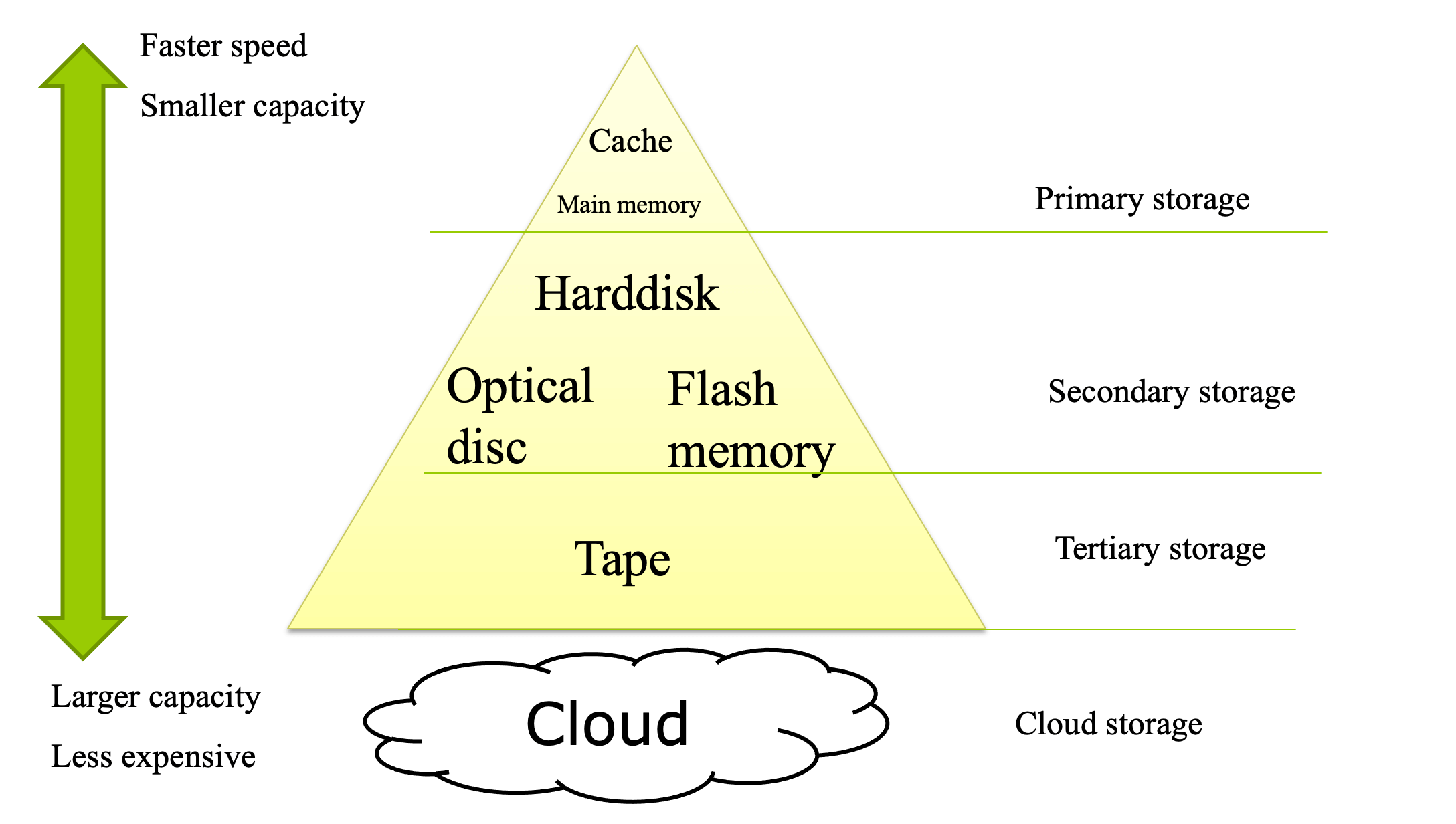
Storage Hierarchy

• Primary storage
  • Fastest media but volatile (cache, main memory).
• Secondary storage
• Next level in hierarchy, non-volatile, moderately fast access time
  • Also called on-line storage, E.g. flash memory, magnetic disks
• Tertiary storage: lowest level in hierarchy, non-volatile, slow access time
  • Also called off-line storage, E.g. magnetic tape, optical storage

Magnetic Disks

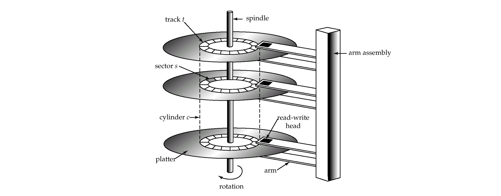
• Read-write head
  • Positioned very close to the platter surface (almost touching it)
  • Reads or writes magnetically encoded information.
• Surface of platter divided into circular tracks
  • Over 16,000 tracks per platter on typical hard disks
• Each track is divided into sectors
  • A sector is the smallest unit of data that can be read or written
  • Sector size typically 512 bytes
  • Typical sectors per track: 200 (on inner tracks) to 400 (on outer tracks)
• To read/write a sector
  • disk arm swings to position head on right track
  • platter spins continually; data is read/written as sector passes under head
• Head-disk assemblies
  • multiple disk platters on a single spindle (typically 2 to 4)
  • one head per platter, mounted on a common arm.
• Cylinder i consists of ith track of all the platters

Performance Measures of Disks

• Access time – the time it takes from when a read or write request is issued to when data transfer begins
  • Seek time – time it takes to reposition the arm over the correct track
    • Average seek time is 1/2 the worst case seek time
      • Would be 1/3 if all tracks had the same number of sectors, and we ignore the time to start and stop arm movement
    • 4 to 10 milliseconds on typical disks
  • Rotational latency – time it takes for the sector to be accessed to appear under the head
    • Average latency is 1/2 of the worst case latency
    • 4 to 11 milliseconds on typical disks (5400 to 15000 r.p.m.)
• Data-transfer rate – the rate at which data can be retrieved from or stored to the disk
  • 4 to 8 MB per second is typical
  • Multiple disks may share a controller, so rate that controller can handle is also important

Optimization of Disk-Block Access

• Block – a contiguous sequence of sectors from a single track
  • data is transferred between disk and main memory in blocks
  • sizes range from 512 bytes to several kilobytes
    • Smaller blocks: more transfers from disk
    • Larger blocks: more space wasted due to partially filled blocks
    • Typical block sizes today range from 4 to 16 kilobytes
• Disk-arm-scheduling algorithms order pending accesses to tracks so that disk arm movement is minimized

Storage Access

• A database file is partitioned into fixed-length storage units called blocks. Blocks are units of both storage allocation and data transfer. Typical size of a block ranges between 4Kb-16Kb
• Database system seeks to minimize the number of block transfers between the disk and memory. We can reduce the number of disk accesses by keeping as many blocks as possible in main memory
• Buffer
  • portion of main memory available to store copies of disk blocks.
• Buffer manager
  • subsystem responsible for allocating buffer space in main memory.

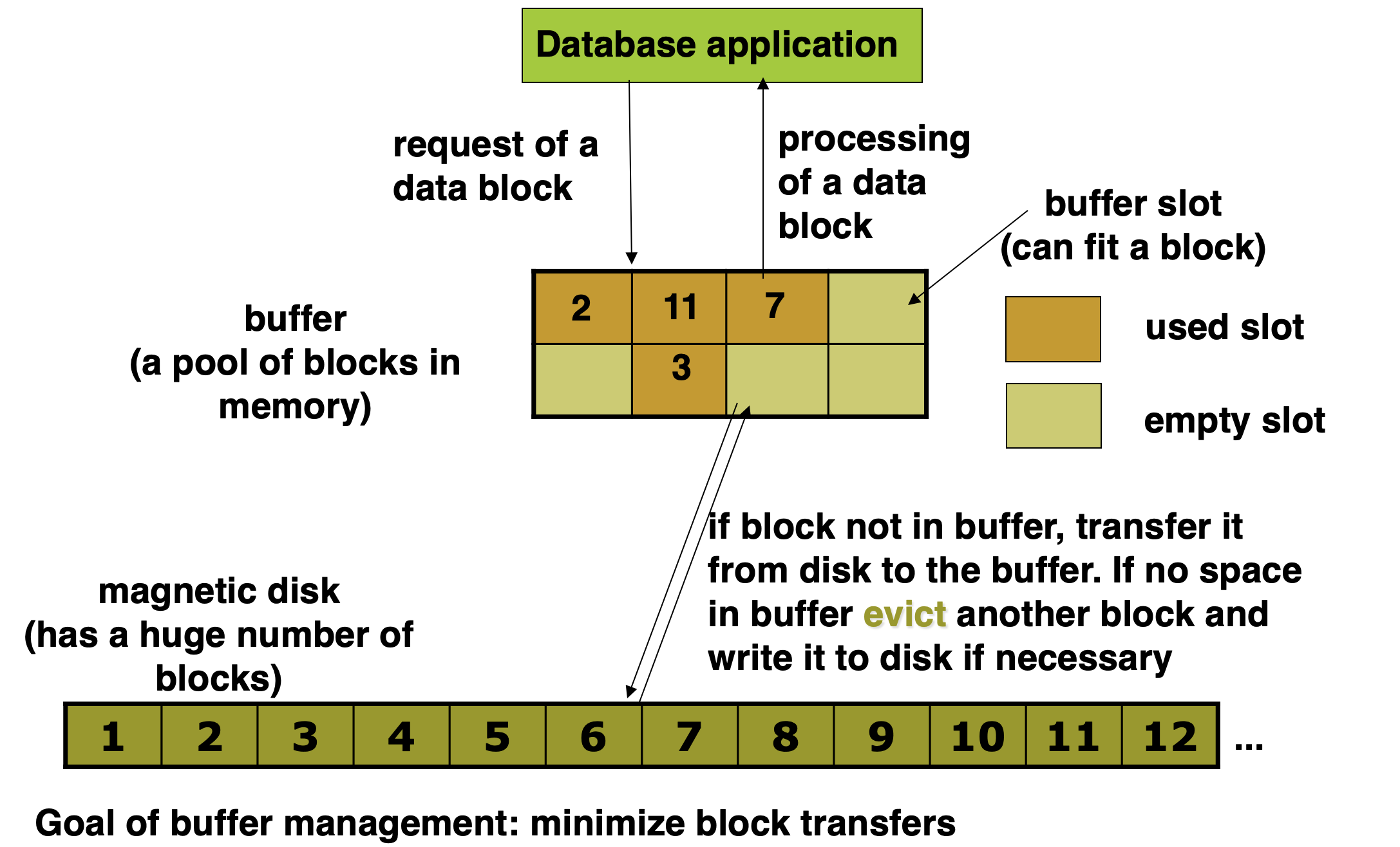
Buffer manager

• Programs call on the buffer manager when they need a block from disk
  • If the block is already in the buffer, the requesting program is given the address of the block in main memory
  • If the block is not in the buffer
    • the buffer manager allocates space in the buffer for the block, replacing (throwing out) some other block, if required, to make space for the new block
    • The block that is thrown out is written back to disk only if it was modified since the most recent time that it was written to/fetched from the disk
    • Once space is allocated in the buffer, the buffer manager reads the block from the disk to the buffer, and passes the address of the block in main memory to requester

Buffer-Replacement Policies

• Most operating systems replace the block least recently used (LRU strategy)
• Idea behind LRU – use past pattern of block references as a predictor of future references. If a block has not been recently used, then it is unlikely that it will be used in the near future
• This replacement policy is also used at different applications. A proxy server keeps in the most recently used web pages in a local cache. If a user requests again a page he has seen, it does not need to be downloaded again in the future
• LRU works well for unpredicted access patterns
• However, queries have well-defined access patterns (such as sequential scans), and a database system can use the information in a user’s query to predict future references
• LRU can be a bad strategy for certain access patterns involving repeated scans of data. Mixed strategy with hints on replacement strategy provided by the query optimizer is preferable

File Organization

• The database is stored as a collection of files. Each file is a sequence of records. A record is a sequence of fields
• Each record has an address in the file, which is called record pointer or record id (simply rid)
• A simple approach
  • assume record size is fixed
  • each file has records of one particular type only
  • different files are used for different relations

Organization of Records in Files

• Heap
  • a record can be placed anywhere in the file where there is space
• Sequential
  • store records in sequential order, based on the value of the search key of each record
• Hashing
  • a hash function computed on some attribute of each record; the result specifies in which block of the file the record should be placed
• Records of each relation may be stored in a separate file. In a clustered file organization records of several different relations can be stored in the same file
  • Motivation: store related records on the same block to minimize I/O
  • However, not good for queries accessing only a few relations
  • In general, this representation is barely used